The Little Learner in Python, Part 5: Automatic Differentiation
Why automatic differentiation matters
Welcome back. Today we will explore automatic differentiation, one of the key technologies behind deep learning. If you have read about neural networks, you have probably encountered backpropagation. It is an application of reverse-mode automatic differentiation, the mode we will implement here.
Think back over the series. In Part 1, we needed an objective function to measure how well a model fit the data. In Part 2, we needed its gradient to update the parameters effectively. In Part 4, we explored several optimizers, but every one of them still needed gradient information.
There are three broad ways to calculate derivatives: numerical differentiation, symbolic differentiation, and automatic differentiation. We have already encountered the expense and approximation errors of numerical differentiation. Symbolic differentiation has its own difficulties, including expressions that can grow unwieldy.
Automatic differentiation applies the chain rule to the operations performed by a program. It avoids finite-difference approximation and does not need to construct one large symbolic derivative. The resulting derivatives are still subject to floating-point arithmetic and the validity of the individual derivative rules, but the approach is well suited to large computations. It is a central capability of frameworks such as PyTorch and TensorFlow that ordinary NumPy does not provide by itself.
This was the concept I spent the most time understanding. My aim here is to make the route gentler than the one I took while reading The Little Learner. We will build the idea one step at a time, then turn it into code.
Gradients and the chain rule
What a gradient means
A derivative tells us how sensitive a function’s output is to a change in its input.
Suppose we have $f(a)$. Increase $a$ by a small amount $\Delta a$ and calculate the new output, $f(a+\Delta a)$. If the output changes by $\Delta f$, we can compare the changes through the ratio:
\[\frac{\Delta f}{\Delta a}\]As $\Delta a$ approaches zero, this ratio approaches the derivative at $a$, provided the derivative exists. For a function with several inputs, a derivative with respect to one input, holding the others fixed, is a partial derivative. The vector of those partial derivatives is the gradient.
Our numerical-differentiation implementation approximated this limiting process with small, finite steps.
Gradients of more complex inputs
For a function $g(a,b)$, consider each input separately:
- Hold $b$ fixed and vary $a$:
- Hold $a$ fixed and vary $b$:
Together, these give the gradient at $(a,b)$:
\[\nabla g = \left(\frac{\partial g}{\partial a},\frac{\partial g}{\partial b}\right)\]The same idea applies when an input is a tensor. Consider changing each scalar element in turn. For a scalar-valued objective, the resulting gradient has the same shape as that input tensor.
For example, let:
\[\mathbf{x}=\begin{bmatrix} x_{11}&x_{12}&x_{13}\\ x_{21}&x_{22}&x_{23} \end{bmatrix}\]If $h(\mathbf{x})$ is a scalar, its gradient with respect to $\mathbf{x}$ is:
\[\nabla_{\mathbf{x}}h=\begin{bmatrix} \frac{\partial h}{\partial x_{11}}&\frac{\partial h}{\partial x_{12}}&\frac{\partial h}{\partial x_{13}}\\ \frac{\partial h}{\partial x_{21}}&\frac{\partial h}{\partial x_{22}}&\frac{\partial h}{\partial x_{23}} \end{bmatrix}\]Remember this rule: for a scalar objective, the gradient with respect to a parameter tensor has the parameter’s shape. With practice, you should be able to look at a parameter’s structure and immediately predict its gradient’s structure.
The chain rule
Now consider a composition, $f(g(a))$. How do we calculate its derivative with respect to the original input $a$?
Break it into stages. Let $b=g(a)$ and $c=f(b)$. Then:
\[\frac{dc}{da}=\frac{dc}{db}\cdot\frac{db}{da}\]We do not need to derive the entire expression at once. We can calculate how each stage responds to its own input, then combine those local derivatives.
This is the key insight: if we know the derivative rules for elementary operations—addition, multiplication, exponentiation, and so on—we can assemble the derivative of a larger computation from those pieces. Automatic differentiation implements this use of the chain rule.
The notation looks as if the two occurrences of $db$ cancel, but that is a mnemonic here, not ordinary cancellation of fractions.
Derivatives of elementary operations
We need a collection of differentiable primitives and their derivative rules.
For addition, $z=a+b$:
\[\frac{\partial z}{\partial a}=1,\qquad\frac{\partial z}{\partial b}=1\]Changing either input by a small amount changes the output by the same amount. The two local derivatives are always $(1,1)$.
For multiplication, $z=ab$:
\[\frac{\partial z}{\partial a}=b,\qquad\frac{\partial z}{\partial b}=a\]Changing only $a$ changes the output by $b\Delta a$; changing only $b$ changes it by $a\Delta b$. The local derivatives are therefore $(b,a)$.
Subtraction can be understood as adding a negative value, and division as multiplying by a reciprocal. Each differentiable primitive supplies another building block.
Computation graphs and the two modes
How do we connect the building blocks? There are two main ways to propagate derivative information: forward mode and reverse mode.
Consider f(g(h(x))). The ordinary value calculation proceeds from the inside out:
Recording the operations and their dependencies gives a computation graph, a directed acyclic graph. It is a graph rather than necessarily a tree because the same input or intermediate value can be reused in several places. In this example, there is only a simple chain. Later, $x$ will feed both $x^2$ and $3x$, and their contributions must be combined.
In forward mode, we calculate values and their derivatives with respect to the chosen input together. A dot marks the derivative with respect to $x$:
\[\dot v_1=\frac{\partial v_1}{\partial x}\] \[\dot v_2=\frac{\partial v_2}{\partial v_1}\dot v_1\] \[\dot v_3=\frac{\partial v_3}{\partial v_2}\dot v_2\]The derivative information travels in the same direction as the value calculation. At the end, $\dot v_3$ is the derivative we want.
In reverse mode, we first calculate the output and retain the information needed for differentiation. Then we propagate derivative information from the output back toward the inputs.
The notation changes for a reason. In forward mode, $\dot v$ means the derivative of $v$ with respect to the input. In reverse mode, we track the derivative of the output with respect to $v$, conventionally written $\bar v$. Confusing these two directions made this topic much harder for me when I first learned it.
The output’s derivative with respect to itself is 1:
\[\bar v_3=\frac{\partial v_3}{\partial v_3}=1\]Then apply the chain rule backward:
\[\bar v_2=\bar v_3\frac{\partial v_3}{\partial v_2},\qquad \bar v_1=\bar v_2\frac{\partial v_2}{\partial v_1},\qquad \bar x=\bar v_1\frac{\partial v_1}{\partial x}\]Both modes give the same final derivative, but they organize the work differently. Forward mode carries derivatives alongside values; reverse mode calculates values first and then propagates derivatives backward. Backpropagation in neural networks follows this reverse-mode pattern.
Reverse mode is especially useful when there are many parameters but one scalar output, such as a loss. An efficiently scheduled reverse pass can obtain all parameter gradients together instead of running a separate forward derivative calculation for each input direction.
A worked example
Let us calculate both the value and derivative of:
\[f(x)=\sin(x^2+3x)\]at $x=2$. Angles are in radians.
Step 1: build the computation graph
Separate the expression into squaring, multiplication by 3, addition, and sine:
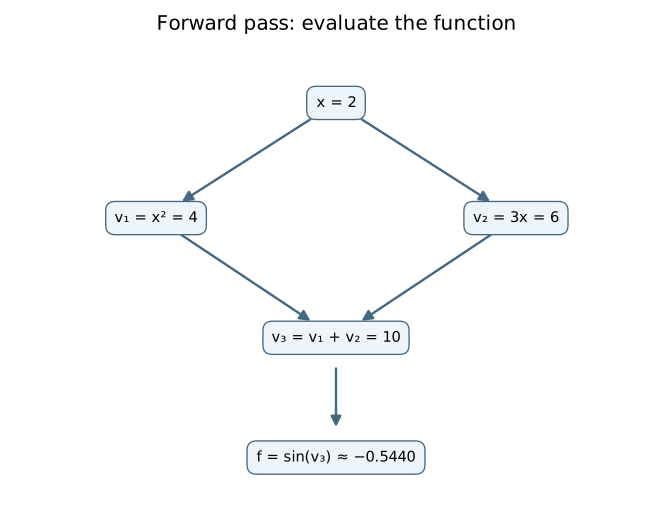
The graph shows the two paths through which $x$ influences the final result.
Step 2: calculate in forward mode
Start with $x=2$ and $dx/dx=1$. Carry the derivative through each operation:
| Operation | Value | Derivative with respect to $x$ |
|---|---|---|
| Input | $x=2$ | $1$ |
| $v_1=x^2$ | $4$ | $2x=4$ |
| $v_2=3x$ | $6$ | $3$ |
| $v_3=v_1+v_2$ | $10$ | $4+3=7$ |
| $v_4=\sin(v_3)$ | $\sin(10)\approx-0.5440$ | $\cos(10)\times7\approx-5.8735$ |
The result is $f(2)\approx-0.5440$ and $f’(2)\approx-5.8735$.
Step 3: calculate in reverse mode
First perform the forward calculation, retaining values and dependencies:
| Recorded operation | Result |
|---|---|
| Square $x$ | $v_1=4$ |
| Multiply $x$ by 3 | $v_2=6$ |
| Add $v_1$ and $v_2$ | $v_3=10$ |
| Take the sine of $v_3$ | $v_4\approx-0.5440$ |
This record is often called a tape. It supplies the information needed for the reverse pass. Our implementation below stores the dependencies in closures rather than a separate list of operation records.
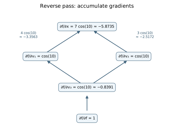
Now propagate the derivatives backward:
- Seed the output with $\partial f/\partial v_4=1$.
- Through sine: $\partial f/\partial v_3=\cos(10)\approx-0.8391$.
- Through addition: the same incoming derivative is passed to both inputs, so $\partial f/\partial v_1=\partial f/\partial v_2\approx-0.8391$.
- Through the two paths to $x$: squaring contributes $\cos(10)\times4\approx-3.3563$, while multiplication by 3 contributes $\cos(10)\times3\approx-2.5172$.
- Add the contributions: $f’(2)=7\cos(10)\approx-5.8735$.
The last step matters: when several paths connect an input to the output, add their derivative contributions. One path must not overwrite another.
Comparing the two modes
Both modes produce the same value and derivative. Reverse mode organizes the calculation into a forward evaluation, a backward propagation of local derivative contributions, and accumulation wherever paths meet.
Implementing System A
We already have tensor operations and optimizers. Until now, scalars were ordinary numbers. To support automatic differentiation, we need values that also remember how to propagate a derivative.
An object-oriented implementation might wrap each value in a class and overload arithmetic operations to record dependencies. That is a familiar way to expose automatic differentiation, but recording the forward calculation and propagating derivatives remain separate jobs.
Following The Little Learner, we will express the dependencies through closures. Each operation produces its value and a function that knows how to send an incoming gradient back to its inputs. The result is a computation graph built out of functions.
We call this implementation System A. The snippets use the Scalar, Tensor, Theta, Callable, and Any names and tensor helpers introduced earlier. They are a step-by-step explanation, not a standalone module; the companion repository provides the assembled implementation.
The data structure
Start with an enhanced scalar:
from dataclasses import dataclass, field
from itertools import count

_id_generator = count()

@dataclass(frozen=True)
class Dual:
    r: Scalar        # The numerical value (real part).
    k: Callable      # A closure that captures the operation's context and propagates gradients.
    id: int = field(default_factory=lambda: next(_id_generator), init=False)
A Dual contains the numerical value r and a link function, k. The link is a closure that remembers the operation’s inputs and the information needed by its derivative rule. Following these links reaches the upstream operations, so the linked closures represent the computation graph.
The unique id gives each node an identity. We use it to accumulate contributions for the same input in a gradient dictionary. It does not, by itself, prevent repeated traversal of a shared subgraph.
Some helpers let us handle ordinary numbers and Dual objects through the same interface:
def is_dual(d: Any) -> bool:
    return isinstance(d, Dual)

def get_r(d: Scalar) -> float:
    return d.r if is_dual(d) else d  # Extract the numerical value from either a plain number or a Dual.

def get_k(d: Scalar) -> Callable:
    return d.k if is_dual(d) else end_of_chain  # Extract the link; plain numbers use end_of_chain.

def is_scalar(d: Any) -> bool:
    return isinstance(d, (int, float)) or is_dual(d)
Differentiable elementary operations
Consider addition:
def add_00(da, db):
    ra, rb = get_r(da), get_r(db)
    result_r = ra + rb  # Forward computation: a + b.

    def link(_result_dual, z, grad_tape) -> None:
        # z is the gradient arriving from downstream (∂L/∂output).
        # Both partial derivatives of addition are 1.
        ga, gb = (z, z)  # Pass the incoming gradient unchanged to both inputs.

        # Call the upstream links recursively to continue backpropagation.
        ka, kb = get_k(da), get_k(db)
        ka(da, ga, grad_tape)
        kb(db, gb, grad_tape)

    return Dual(result_r, link)
First calculate the ordinary sum. Then define link, which captures both inputs.
Of its three arguments, z drives the backward calculation: it is the derivative arriving from downstream, with respect to this operation’s output. grad_tape is a dictionary shared by the whole backward traversal. _result_dual is unused here but keeps the link interface consistent.
The link does two things:
- Apply the local derivative rule to the incoming gradient.
- Call the inputs’ links to continue propagating upstream.
Addition passes z unchanged to both inputs. The link does not store their gradients in the dictionary itself; it sends the contributions upstream. The leaf links will accumulate them.
Multiplication follows the same structure with a different rule:
def mul_00(da, db):
    ra, rb = get_r(da), get_r(db)
    result_r = ra * rb  # Forward computation: a * b.

    def link(_result_dual, z, grad_tape) -> None:
        # The gradient rule for multiplication:
        # ∂(a*b)/∂a = b, ∂(a*b)/∂b = a
        # Multiply by the downstream gradient z (the chain rule).
        ga, gb = (rb * z, ra * z)

        ka, kb = get_k(da), get_k(db)
        ka(da, ga, grad_tape)
        kb(db, gb, grad_tape)

    return Dual(result_r, link)
At a leaf node, there is nowhere further to propagate. We simply accumulate the contribution:
# A leaf link follows the same interface but stops propagation.
def end_of_chain(d: Scalar, z: float, grad_tape: dict) -> None:
    # There is no gradient to record for a plain numerical value.
    if is_dual(d):

        dg = grad_tape.get(d.id, 0.0)
        grad_tape[d.id] = dg + z

def make_dual(d: Scalar) -> Dual:
    """Create a leaf Dual whose link is end_of_chain."""
    return Dual(get_r(d), end_of_chain)
Notice dg + z. This is addition, not replacement. In our worked example, $x$ receives contributions through both $x^2$ and $3x$. The final addition of those two contributions happens at this line.
Factoring out the pattern: prim1 and prim2
Addition, multiplication, exponentiation, and logarithms all follow the same pattern: calculate a value, then construct a link. We can write two higher-order functions for unary and binary primitives:
def prim2(primal_fn: Callable, derivative_fn: Callable) -> Callable:
    """
    Construct a differentiable version of a binary operation.
    primal_fn: the forward calculation, such as lambda a, b: a + b.
    derivative_fn: returns the input gradients (dL/da, dL/db).
    """
    def primitive(da, db):
        ra, rb = get_r(da), get_r(db)
        result_rho = primal_fn(ra, rb)

        # If neither input is a Dual, return the numerical result directly.
        # Avoid allocating link closures when no gradient is needed.
        if not is_dual(da) and not is_dual(db):
            return result_rho

        def link(d, g, grad_tape) -> None:
            ga, gb = derivative_fn(ra, rb, g)  # Calculate the input gradients.
            # Intermediate gradients need not be stored; end_of_chain accumulates leaf gradients.
            ka, kb = get_k(da), get_k(db)
            ka(da, ga, grad_tape)  # Continue propagating to a.
            kb(db, gb, grad_tape)  # Continue propagating to b.

        return Dual(result_rho, link)
    return primitive

# Unary operations follow the same pattern.
def prim1(primal_fn: Callable, derivative_fn: Callable) -> Callable:

    def primitive(da):

        ra = get_r(da)
        result = primal_fn(ra)

        if not is_dual(da):
            return result

        def link(d, g, grad_tape) -> None:
            ga = derivative_fn(ra, g)

            ka = get_k(da)
            ka(da, ga, grad_tape)
        return Dual(result, link)

    return primitive
The early return avoids building a graph when no input needs differentiation. With these helpers, the primitive definitions become concise:
import math

# Binary operations.
add_00 = prim2(lambda a,b: a+b, lambda a,b,z: (z, z))
mul_00 = prim2(lambda a,b: a*b, lambda a,b,z: (b*z, a*z))
div_00 = prim2(
    lambda ra, rb: ra / rb,
    lambda ra, rb, z: (z / rb,-ra * z / (rb**2)) # d/da (a/b) = 1/b, d/db (a/b) = -a/b^2
)
sub_00 = prim2(
    lambda ra, rb: ra - rb,
    lambda ra, rb, z: (z, -z)  # d/da (a-b) = 1, d/db (a-b) = -1
)

# Unary operations.
exp_0 = prim1(lambda a: math.exp(a), lambda a,z: math.exp(a)*z)
log_0 = prim1(lambda a: math.log(a), lambda a,z: z/a)

def pow_n(n: float):
    return prim1(
        lambda ra: ra**n,
        lambda ra, z: n * (ra ** (n - 1)) * z # d/da (a^n) = n*a^(n-1)
    )

square_0 = pow_n(2.0)

sqrt_0 = prim1(
    lambda ra: math.sqrt(ra),
    lambda ra, z: 0.5 * z / math.sqrt(ra),  # d/da sqrt(a) = 0.5 / sqrt(a)
)
Each rule still has the usual mathematical domain restrictions: logarithms require positive real inputs, division needs a nonzero denominator, and the displayed square-root derivative is singular at zero.
Use ext1 and ext2 to lift these scalar operations over tensors represented as nested lists:
tsqr = ext1(square_0, 0)
tsqrt = ext1(sqrt_0, 0)
tlog = ext1(log_0, 0)
texp = ext1(exp_0, 0)

tsub = ext2(sub_00, 0, 0)
tmul = ext2(mul_00, 0, 0)
tadd = ext2(add_00, 0, 0)
tdiv = ext2(div_00, 0, 0)
Extracting gradients: nabla and get_grad
Once a computation uses these enhanced operations, its closures retain the dependencies needed for backpropagation. We can then extract the gradients of the inputs we care about:
def get_grad(y: Dual, wrt: Theta) -> Theta:
    """Extract the gradients of output y with respect to wrt."""
    sigma = {}               # Map leaf IDs to gradients; the graph itself lives in the chain of closures.
    get_tape(y, sigma)          # Start backpropagation and fill sigma.

    return [sigma.get(d.id, 0.0) for d in wrt]   # Return gradients in the order of this flat list of scalar parameters.
get_tape starts the backward propagation:
def get_tape(y: Dual | list[Dual], grad_tape: dict) -> None:
    if is_scalar(y):
        k = get_k(y)
        k(y, 1.0, grad_tape)  # Start at the output with a gradient of 1.0.
    elif isinstance(y, list):
        for item in y:
            get_tape(item, grad_tape)
Finally, replace numerical differentiation with the new nabla:
def nabla(f: Callable, theta: Theta):
    # 1. Wrap the input parameters as Duals to enable differentiation.
    wrt = [make_dual(t) for t in theta]
    # 2. Evaluate the function, building the computation graph.
    result = f(wrt)
    # 3. Backpropagate and extract the gradients.
    return get_grad(result, wrt)
This compact version wraps and extracts a flat list of scalar parameters. The tensor arithmetic can operate on nested lists, but these particular nabla and get_grad snippets do not recursively wrap and extract a nested parameter set. The complete repository implementation handles that additional traversal.
Also note the meaning of a list-valued output: get_tape seeds every output element with 1. The result is the gradient of their sum, not a full Jacobian. This is useful for loss contributions that should be added together.
The closure-based traversal prioritizes clarity. A shared intermediate can be visited through several paths; a production engine normally schedules accumulation so that shared work is not needlessly repeated. The essential derivative rule remains the same: multiply along a path and add contributions from different paths.
Summary and what comes next
Automatic differentiation breaks a computation into elementary operations and combines their derivative rules through the chain rule. We have turned that idea into System A: scalar values accompanied by closures that know how to propagate gradients.
System B will address some of its performance costs by moving from scalar nodes to tensor nodes. I originally intended to include that implementation here, but the concepts deserve room to breathe. The next article, Automatic Differentiation 2.0, explains the tensor-level approach and the further gains from vectorized computation.
After that, we will use the engine to train a neural network of our own.
Previous: Part 4: Optimizers.
Next: Part 5.5: Automatic Differentiation 2.0.
Series: The Little Learner in Python.