The Little Learner in Python, Part 4: Optimizers
Introduction: why optimizers matter
Welcome back. The first three articles introduced linear models, implemented gradient descent, and developed tensor operations. With large datasets and many parameters, however, full-batch gradient descent can become slow and difficult to tune. Researchers have developed several improvements, packaged as optimizers, to make training more practical.
This article follows four ideas:
- Stochastic gradient descent (SGD): learn from samples instead of processing the entire dataset at every step.
- Momentum: carry information from earlier updates into the next one.
- RMSProp: adapt update sizes using recent squared gradients.
- Adam: combine momentum with adaptive scaling.
The examples build on the nested-list tensor functions from Part 3, not its separate NumPy comparison sketch. They also use the earlier revise helper.
Stochastic gradient descent: working with large datasets
The cost of full-batch computation
Our earlier implementation uses the whole dataset to calculate each gradient. The relevant operations look like this, with objective_func and theta standing for the current objective and parameters:
plane_objective = l2_loss(plane)(plane_xs, plane_ys) # Define an objective.
gradient = nabla(objective_func, theta)  # Calculate a gradient.
The objective is a closure with access to the complete dataset. When that dataset is large, even one gradient calculation can be expensive. Imagine a farmer who wants to know whether a box of apples is ripe and tastes every apple before deciding.
Learning from a random sample
The farmer would normally taste a few randomly selected apples instead. One sample can be misleading, but repeated samples give useful information at a much lower cost.
We can apply the same idea to gradient descent by using a randomly selected subset of the data:
# Use random for sampling.
import random

def sampling_obj(
    full_objective: Callable,  # Objective builder for a dataset.
    xs: Tensor,                # All input data.
    ys: Tensor,                # All target data.
    batch_size: int = 32       # Mini-batch size, a hyperparameter.
) -> Callable:
    """Create an objective that samples a mini-batch at each evaluation."""
    n = len(xs)

    def minibatch_objective(theta: Theta):
        # Choose random batch indices.
        batch_indices: list[int] = random.sample(range(n), batch_size)

        # Build the mini-batch.
        xs_batch = [xs[i] for i in batch_indices]
        ys_batch = [ys[i] for i in batch_indices]

        # Create an objective for that batch.
        batch_objective = full_objective(xs_batch, ys_batch)

        return batch_objective(theta)

    return minibatch_objective

# Example usage.
plane_simple_objective = sampling_obj(l2_loss(plane), plane_xs, plane_ys, 4)
The closure retains the complete dataset, but each evaluation passes only a random subset to the underlying objective builder, here l2_loss(plane). batch_size must not exceed the dataset length because random.sample samples without replacement.
Using sampled gradients gives us stochastic gradient descent. More precisely, the version above uses a mini-batch; strictly speaking, SGD can refer to the one-sample case, although the name is often used for mini-batch training too.
There is an important interaction with our current numerical-gradient implementation. Do not pass this resampling objective directly to finite-difference nabla and expect a valid mini-batch gradient. nabla compares a baseline loss with perturbed losses. If every call draws a new batch, those differences include changes in the data as well as changes in the parameter. Dividing that unrelated variation by a tiny delta can produce enormous, meaningless estimates.
For numerical differentiation, choose the batch once per optimizer step, build a fixed objective from it, and use that same objective for every evaluation in the gradient calculation. The example above shows the sampling idea, but the optimizer loop below does not implement that batch-freezing step. Automatic differentiation avoids subtracting separately sampled loss evaluations, but randomness still needs to be handled in a way the chosen library supports.
What SGD changes
For an objective whose evaluation cost scales with the number of examples, using a batch of size $B$ instead of a dataset of size $N$ reduces that part of the per-step work from $O(N)$ to $O(B)$. This does not remove the separate parameter-dependent cost of our numerical differentiation.
Sampling introduces gradient noise. That noise can sometimes help an optimizer move away from poor regions, but it does not guarantee escape from every local minimum.
Batch size involves a trade-off: smaller batches are cheaper per step but noisier; larger batches usually give a more representative estimate at a higher memory and computation cost. Our loss is a sum, so changing batch size also changes the typical gradient scale. Keep that in mind when comparing learning rates across batch sizes.
Making gradient descent modular
Before adding more optimizers, let us reorganize the implementation.
Our gradient-descent function currently encloses an update function and uses revise to apply it repeatedly. The main difference between optimizer variants is the update rule. We can separate that rule from the shared loop.
Some rules need more than the current parameter value. They also maintain information such as velocity or a running average. We therefore introduce two additional operations: one to wrap a parameter together with its optimizer state, and another to extract the parameter again.
# Collect the growing number of hyperparameters in a configuration class.
class GDConfig:
    """Gradient-descent configuration defaults.
    Attributes:
        lr: learning rate (default 0.01).
        revs: number of updates (default 200).
        batch_size: mini-batch size (default 4).
    """
    lr: float = 0.01
    revs: int = 200
    batch_size: int = 4

def gradient_descent_builder(
    inflate,   # Wrap a parameter in optimizer-specific state.
    deflate,   # Extract the parameter from that state.
    update     # Apply the optimizer's update rule.
):
    """
    Optimizer factory.
    Return an optimizer built from the supplied state and update functions.
    """
    def optimizer(objective: Callable, initial_theta: Theta, hyper: GDConfig):

        # Wrap each initial parameter.
        initial_inflated_theta = [inflate(param) for param in initial_theta]

        # Define one revision step for the parameter set.
        def revision_step(inflated_theta: Any):

            # Extract the current parameters.
            theta = [deflate(P) for P in inflated_theta]

            # Calculate gradients.
            gradients = nabla(objective, theta, delta=1e-6)

            # Update each parameter and its associated state.
            next_inflated_theta = [
                update(p, g, hyper) for p, g in zip(inflated_theta, gradients)
            ]

            # Return the updated parameter states.
            return next_inflated_theta

        # Repeat the revision step.
        final_inflated_theta = revise(revision_step, hyper.revs, initial_inflated_theta)

        # Extract and return the final parameters.
        return [deflate(p) for p in final_inflated_theta]

    # Return the constructed optimizer.
    return optimizer
The returned optimizer plays the role of the earlier gradient_descent function. revision_step handles the shared work of extracting parameters and calculating gradients; update now handles only one parameter’s update rule and associated state.
As discussed in Part 3, each parameter is a tensor, but the complete parameter set may contain tensors of different shapes. We therefore pass each parameter and its corresponding gradient to update separately.
The configuration class provides default attributes. In this small implementation, the later dataclass subclasses only generate constructor fields for their own declared fields: inherited lr, revs, and batch_size are not automatically constructor arguments. Also, batch_size is descriptive configuration here; the factory itself does not perform sampling.
We can now recreate basic gradient descent:
# Identity wrapping and extraction.
def naked_i(p: P) -> P: return p
def naked_d(p: P) -> P: return p

# Basic update: theta = theta - alpha * gradient.
def naked_u(p: Tensor, g: Tensor, hyper: GDConfig):
    return tsub(p, tmul(g, hyper.lr))

# Build the basic optimizer.
naked_gd = gradient_descent_builder(naked_i, naked_d, naked_u)
Momentum
Imagine four brothers running a relay. The first is fast, the next two are slower, and the last is very slow. Their coach suggests that each runner keep hold of the baton briefly while handing it over, pulling the next runner forward and passing along some speed.
In the optimization analogy, the runners are successive updates. Keeping hold of the baton means carrying some of the previous update into the next one. Even if the current gradient becomes smaller, accumulated motion can keep the parameters moving.
This resembles physical momentum. The optimizer maintains a velocity that combines previous motion with the current gradient. A momentum coefficient, often 0.9, controls how much of the previous velocity remains.
Implementing momentum
from collections import namedtuple
from dataclasses import dataclass

VelocityP = namedtuple("VelocityP", ["parameter", "velocity"])

@dataclass(frozen=True)
class MGDConfig(GDConfig):
    momentum: float = 0.9  # Momentum coefficient, often written as mu or beta_1.

def velocity_i(p: P) -> VelocityP:
    """Initialize a parameter with zero velocity."""
    return VelocityP(p, zeros(p))

def velocity_d(vp: VelocityP) -> P:
    """Extract the parameter."""
    return vp.parameter

def velocity_u(vp: VelocityP, g: Tensor, h: MGDConfig) -> VelocityP:
    """Momentum update:
    1. Update velocity: v = mu * v_old - alpha * gradient.
    2. Update the parameter: theta = theta + v.
    """
    v = tsub(tmul(h.momentum, vp.velocity), tmul(h.lr, g))
    p = tadd(vp.parameter, v)
    return VelocityP(p, v)

# Build the momentum optimizer.
mgd = gradient_descent_builder(velocity_i, velocity_d, velocity_u)
Understanding the momentum equations
Write the update in three steps:
\[v = \mu v_{\text{old}} - \alpha \nabla J(\theta_{\text{old}})\] \[\theta_{\text{new}} = \theta_{\text{old}} + v\] \[\theta_{\text{new}} = \theta_{\text{old}} - \alpha \nabla J(\theta_{\text{old}}) + \mu v_{\text{old}}\]The last equation is ordinary gradient descent plus the retained velocity, $\mu v_{\text{old}}$. Here, velocity is accumulated, signed update information, already scaled by the learning rate. When gradients keep pointing in a similar direction, successive updates reinforce one another. When the direction changes, that accumulated motion takes time to slow or reverse.
The coefficient $\mu$, called momentum in the code, controls the weight of this history. At $\mu = 0$, the rule reduces to basic gradient descent, or SGD if the gradients come from sampled data. Values closer to 1 retain more history, which can accelerate progress but also increase overshoot.
Another common formulation keeps an exponential moving average, or EMA, of the gradients:
\[v_t = \mu v_{t-1} + (1-\mu)\nabla J(\theta_{t-1})\] \[\theta_t = \theta_{t-1} - \alpha v_t\]This form makes the weighting of old and new information explicit. The two formulations are not equivalent at the same learning rate. The EMA scales new gradients by the extra factor $1-\mu$. With zero initial state and matched gradient histories, matching the first formulation requires increasing the EMA formulation’s learning rate by $1/(1-\mu)$. At $\mu = 0.9$, that is a factor of 10.
This EMA form, with its $1-\beta$ factor, is also used for Adam’s first-moment estimate. Understanding it now will make Adam easier to follow.
What momentum changes
Momentum combines the current gradient with previous motion. It can accelerate updates along a consistent direction and smooth some oscillations. In a favorable problem, it may reach a useful solution in hundreds of iterations where basic gradient descent needs thousands; the improvement depends on the problem and settings.
The parameter trajectory illustrates the effect:
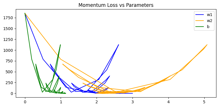
Accumulated velocity can carry the parameters past a minimum or make them oscillate around it. It can also carry them through shallow local dips. Momentum is useful, but more retained motion is not always better.
RMSProp: adaptive scaling
Basic gradient descent and the momentum rule above use one base learning rate for every parameter. But different components can have very different gradient scales. A component with consistently large gradients may need a smaller effective step, while another with small gradients may benefit from a larger one.
RMSProp, short for Root Mean Square Propagation, addresses this by keeping an elementwise moving average of squared gradients. It divides the base learning rate by the square root of that average, plus a small stability constant.
Implementing RMSProp
@dataclass(frozen=True)
class RMSPropConfig(GDConfig):
    decay: float = 0.9    # Decay rate for the squared-gradient average.
    eps: float = 1e-8     # Numerical stability constant.

# State: parameter plus a running average of squared gradients.
RmsP = namedtuple("RmsP", ["parameter", "running_avg"])

def rms_i(p: P) -> RmsP:
    """Initialize with a zero running average."""
    return RmsP(p, zeros(p))

def rms_d(rms_p: RmsP) -> P:
    """Extract the parameter."""
    return rms_p.parameter

def smooth(decay: float, average: Tensor, g: Tensor) -> Tensor:
    """EMA: decay * old_average + (1 - decay) * g; RMSProp passes squared gradients as g."""
    return tadd(tmul(decay, average), tmul(1 - decay, g))

def rms_u(rms_p: RmsP, g: Tensor, h: RMSPropConfig) -> RmsP:
    """RMSProp update:
    1. Update the average: r = beta * r_old + (1 - beta) * (g * g).
    2. Effective learning rate: lr_eff = alpha / (sqrt(r) + epsilon).
    3. Update the parameter: theta = theta - lr_eff * g.
    """
    r = smooth(h.decay, rms_p.running_avg, tsqr(g))
    new_lr = tdiv(h.lr, tadd(tsqrt(r), h.eps))
    p = tsub(rms_p.parameter, tmul(new_lr, g))
    return RmsP(p, r)
Use gradient_descent_builder(rms_i, rms_d, rms_u) to assemble this rule into an optimizer, just as we did for momentum.
Understanding the RMSProp equations
The rule is:
\[r_t = \beta r_{t-1} + (1-\beta)\bigl(\nabla J(\theta_{t-1})\bigr)^2\] \[\theta_t = \theta_{t-1} - \frac{\alpha}{\sqrt{r_t}+\epsilon}\nabla J(\theta_{t-1})\]The arithmetic on tensor components is elementwise. Start with the familiar gradient-descent update and replace the fixed learning rate with a changing scale. We want that scale to decrease when recent gradients are large and increase when they are small. A reciprocal gives us that relationship. Adding $\epsilon$ prevents a zero denominator.
That explains the effective learning rate $\alpha/(\sqrt{r_t}+\epsilon)$, called new_lr in the code. Why use a moving average of squared gradients? Dividing directly by the current gradient would cancel its magnitude: $(\alpha/g)g = \alpha$. Instead, the moving average reflects recent gradient sizes and smooths individual fluctuations.
The decay coefficient $\beta$, often 0.9 for RMSProp, controls the weight of earlier squared gradients. Its role resembles the momentum coefficient, but it tracks a different quantity. In Adam, the two coefficients are conventionally distinguished as $\beta_1$ and $\beta_2$.
Squaring removes the sign before averaging; taking the square root brings the scale back to that of a gradient. The direction of the final update still comes from the current gradient.
What adaptive scaling changes
Adaptive scaling can reduce the imbalance between parameter components whose gradients have different magnitudes. It does not guarantee that all parameters converge at the same speed or that one optimizer will always be more stable than another.
The illustration shows the smoother trajectory obtained in this example:
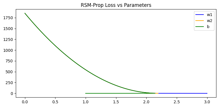
On some problems RMSProp requires more steps than a well-tuned alternative; on others, its response to changing gradient scales is useful. The figure is an example of behavior, not a universal ranking.
Adam: combining the two ideas
Adam, short for Adaptive Moment Estimation, combines momentum with adaptive scaling. It maintains an average of gradients—the first moment—and an average of squared gradients—the second raw moment. The latter is not the centered variance, which would subtract the squared mean.
The basic sequence is:
- Update the first-moment estimate.
- Update the second-moment estimate.
- Use the second estimate to scale the step.
- Update the parameter using the first estimate.
@dataclass(frozen=True)
class AdamConfig(GDConfig):
    decay: float = 0.999    # Second-moment decay rate, beta_2.
    momentum: float = 0.9   # First-moment decay rate, beta_1.
    eps: float = 1e-8       # Numerical stability constant.

# State: parameter, first moment, and second raw moment.
AdamP = namedtuple("AdamP", ["parameter", "velocity", "running_avg"])

def adam_i(p: P) -> AdamP:
    """Initialize both moment estimates to zero."""
    return AdamP(p, zeros(p), zeros(p))

def adam_d(adam_p: AdamP) -> P:
    """Extract the parameter."""
    return adam_p.parameter

def adam_u(adam_p: AdamP, g: Tensor, h: AdamConfig) -> AdamP:
    """Simplified Adam update without bias correction:
    1. First moment: v = beta_1 * v_old + (1 - beta_1) * g.
    2. Second moment: r = beta_2 * r_old + (1 - beta_2) * (g * g).
    3. Effective learning rate: lr_eff = alpha / (sqrt(r) + epsilon).
    4. Update the parameter: theta = theta - lr_eff * v.
    """
    v = smooth(h.momentum, adam_p.velocity, g)
    r = smooth(h.decay, adam_p.running_avg, tsqr(g))
    new_lr = tdiv(h.lr, tadd(tsqrt(r), h.eps))
    p = tsub(adam_p.parameter, tmul(new_lr, v))
    return AdamP(p, v, r)

# Build the simplified Adam optimizer.
adam_gd = gradient_descent_builder(adam_i, adam_d, adam_u)
The full Adam algorithm also corrects the initial bias caused by starting both moving averages at zero. At step $t$, it divides the first moment by $1-\beta_1^t$ and the second by $1-\beta_2^t$. The simplified implementation here omits bias correction, so its early updates differ from standard Adam implementations in libraries such as PyTorch.
Adam combines useful features of momentum and RMSProp, and its commonly used coefficients, $\beta_1=0.9$ and $\beta_2=0.999$, provide a starting point for many problems. Adam and variants such as AdamW and Nadam are widely used, but their performance still depends on the task and tuning.
In the examples that motivated this article, Adam’s trajectory looked similar to RMSProp’s and converged faster, while momentum was faster still. Treat that ordering as an observation about those examples, not a general property of the algorithms.
Summary
We have moved from basic full-batch gradient descent to four useful ideas:
- SGD and mini-batches reduce the amount of data processed in each update.
- Momentum carries information from previous updates into the next one.
- RMSProp scales each component using its recent squared gradients.
- Adam combines a gradient average with squared-gradient scaling.
Understanding what each optimizer tracks helps us diagnose and debug training rather than treating the optimizer as a black box.
You will probably want to run the code now. If training produces inf or NaN, investigate the actual source instead of assuming that the optimizer has become “too good.” In this implementation, one concrete problem is the combination of resampling on every objective call with finite differences, described earlier. Excessive step sizes and numerical errors can also destabilize training. A small loss or gradient does not, by itself, prove that an adaptive update must explode; the update depends on both its numerator and denominator, including $\epsilon$.
Automatic differentiation removes finite-difference approximation and its repeated perturbed evaluations. You can experiment with a compatible implementation such as JAX’s grad, but its inputs, operations, and handling of randomness must be adapted appropriately. It is not a guarantee against every numerical failure.
If you would rather build the mechanism yourself, the next article introduces automatic differentiation—one of the most important and interesting parts of this series.
Previous: Part 3: Tensors.