The Little Learner in Python, Part 1: The Core Optimization Mechanism
The Little Learner
Welcome to this exploration of deep learning. After studying its foundations systematically, I decided to write a series of posts sharing what I learned. We will start with basic concepts, work toward the principles and practice of deep neural networks, and ultimately build a small deep-learning framework. The series is intended both for newcomers and for readers who want to strengthen their foundations.
The main source is The Little Learner: A Straight Line to Deep Learning. Two things drew me to this distinctive introduction: its Socratic teaching style, which builds understanding through questions and answers, and its use of functional programming in Scheme.
Neither the teaching style nor the language is mainstream, but those qualities are part of why I love the book. In these posts, I will replace the dialogue with direct explanations and use Python, the dominant language in deep learning, instead of Scheme. Two characteristics of the book will remain:
- A simple starting point. I will not assume much mathematical background. Working through the series should also make later study of calculus, linear algebra, and probability easier.
- A mainly functional programming style. Although we are not using Scheme, we will retain the functional approach. If closures and higher-order functions are unfamiliar, it is worth learning the basics first.
Why keep the functional style? Partly personal preference. More practically, functional programming aims to minimize side effects and pass data through functions, making data flow easier to follow and reason about. Deep learning involves many mathematical expressions and data transformations, which fit this approach well. Functional ideas also appear in libraries such as JAX and PyTorch.
Some preparation will help:
- Basic Python: list comprehensions, anonymous functions, and higher-order functions.
- Basic mathematics: concepts such as linear functions. We will develop the other ideas we need along the way.
- An open mind: the prose and code may feel unfamiliar. Each post covers roughly three or four chapters of the book, so there is quite a lot to absorb. I will inevitably make mistakes, too. Think through the examples, run the code, try debugging problems yourself, and feel free to contact me with feedback.
Ready? Let us begin.
A simple linear function
Recall the straight-line functions from school mathematics: $f(x) = wx + b$, or $y = kx + b$. Writing $f(x)$ emphasizes that this is a function; writing $y$ emphasizes the resulting value. The choice of letter for the coefficient makes no mathematical difference. In machine learning, we usually use $w$ for weight and $b$ for bias.
With $w = 1$ and $b = 0$, the relationship looks like this:
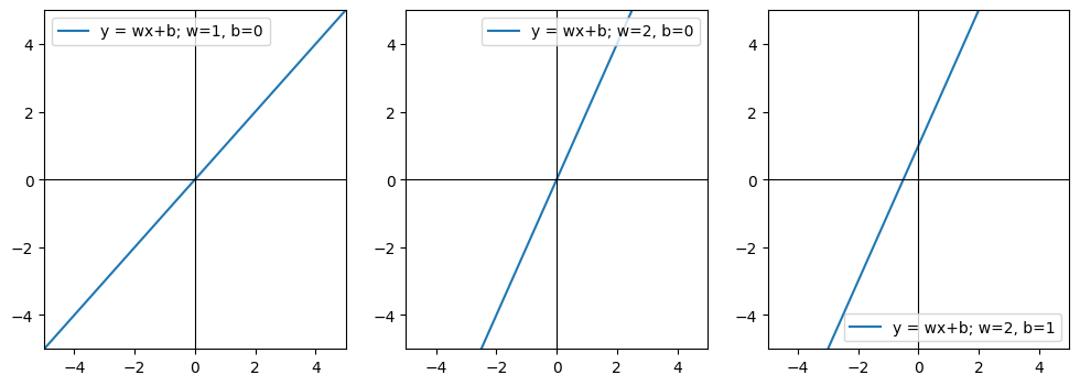
When the relationship between the independent variable $x$ and dependent variable $y$ forms a straight line in Cartesian coordinates, we call it a linear function in this context. The weight $w$ determines the slope: how quickly $y$ changes as $x$ changes. The bias $b$ shifts the whole line up or down. Keep those roles in mind, because these are the two values we will learn.
Here is a representation in code:
from typing import Callable, Iterable, List

# The values are real numbers; use float to represent them.

def line(x: float) -> Callable[[float, float], float]:

    return lambda w, b: w * x + b
line is a higher-order function: calling it returns another function, in this case an anonymous one. The returned function takes w and b and uses them, together with the captured x, to calculate the output.
If this style is unfamiliar, you can initially think of it as a function with three inputs: x, w, and b. We separate them because later code will handle input data differently from weights and biases.
For example, suppose w=1, b=0, and we want the output for x=2. First pass 2 to line, then pass 1 and 0 to the function it returns:
result = line(2)(1, 0)  # result = 2
print(result)  # Output: 2
The problem
In school mathematics, we often work with known coefficients and solve for a variable. Machine learning usually poses a different problem: given some values of $x$ and $y$, learn or estimate $w$ and $b$.
Here, $x$ is the independent variable, or input, and $y$ is its corresponding output. In code, the input is passed as an argument and the prediction is returned by the function.
The collection of input-output pairs is a dataset. One input and its corresponding output form a data point, or sample. The values $w$ and $b$ are the model’s parameters. Together, they form the parameter set, commonly written as the Greek letter $\theta$, pronounced “theta.” In this example, $\theta = [w, b]$.
Suppose our inputs are $[2.0, 1.0, 4.0, 3.0]$, and the corresponding outputs are $[1.8, 1.2, 4.2, 3.3]$. We want to infer $w$ and $b$ from these data.
We can plot the points:
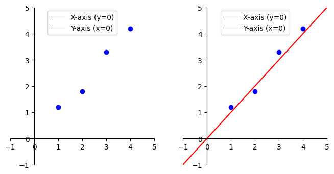
It is easy to imagine a straight line through this cluster and estimate its weight and bias by eye. But how can we turn that visual process into a program that a computer can execute?
An approach
One approach is successive approximation, or iterative optimization. Start with a guess for $w$ and $b$, compare the predicted outputs with the observed outputs, and repeatedly adjust the parameters to reduce the discrepancy.
Suppose we choose $\theta = [0.0, 0.0]$. For the point $(x=2.0, y=1.8)$, the prediction line(2.0)(0.0, 0.0) is 0.0. We commonly write a prediction as $\hat{y}$, pronounced “y-hat,” to distinguish it from the observed $y$. The difference is $1.8 - 0 = 1.8$.
This gives us a first, rough measure of prediction error. A loss, or cost, measures how poorly the current parameters fit the data. In this article, I use the terms interchangeably when discussing the objective over a dataset; other materials distinguish a loss for one sample from a cost aggregated over the dataset.
We can write a function to calculate the signed error for one input under a given parameter set:
def loss_single(x: float, y: float, theta: list[float]) -> float:

    pred_y = line(x)(*theta)
    return y - pred_y
Improving the loss function
This initial version has several problems.
First, it processes one value at a time. We want it to handle the whole dataset, so we need to rewrite line. Second, we want a single number that measures the overall error, rather than a list of separate errors. Let us begin by adding them together:
# Let line process a collection of inputs rather than a single value.
def line(xs: Iterable[float]) -> Callable[[float, float], List[float]]:

    return lambda w, b: [w * x + b for x in xs]

# A helper for elementwise vector subtraction:
# [a, b] - [c, d] = [a - c, b - d], and so on.
def sub(ms: Iterable[float], ns: Iterable[float]) -> List[float]:

    return [m - n for m, n in zip(ms, ns)]

def loss(xs: Iterable[float], ys: Iterable[float], theta: list[float]):

    pred_ys = line(xs)(*theta)
    errors = sub(ys, pred_ys)
    return sum(errors)
The function now returns one total, but it introduces another problem. With our definition y - pred_y, a prediction that is too high produces a negative error, while one that is too low produces a positive error. Those errors can cancel, making the total look small even when individual predictions are inaccurate.
We need to prevent that cancellation. Two options are to take each error’s absolute value or to square it. These give us absolute-error loss, commonly called L1 loss, and squared-error loss, commonly called L2 loss in this setting. Each has its uses. We will use squared errors here.
For the complete dataset, we can calculate the sum of squared errors as follows:
# Square every value in an iterable.
def sqr(xs: Iterable[float]) -> List[float]:

    return [x ** 2 for x in xs]

def l2_loss(xs: Iterable[float], ys: Iterable[float], theta: List[float]) -> float:

    pred_ys = line(xs)(*theta)
    errors = sub(ys, pred_ys)
    sqr_err = sqr(errors)
    loss = sum(sqr_err)
    return loss
Our goal is to find a parameter set $\theta$ that minimizes this total squared error. We repeatedly evaluate the loss and use it to guide parameter changes. The function we are minimizing is called the objective function, sometimes written as $J$.
There are two more things to improve. We do not want to pass the same dataset every time we update $\theta$. Also, l2_loss currently calls line directly, tying it to that particular model. We want a loss function that can work with different models.
Higher-order functions solve both problems. We supply the model and dataset first, then get back an objective that needs only $\theta$. The returned function retains access to the model and data through a closure:
def l2_loss(target: Callable[[Iterable[float]], Callable[[float, float], List[float]]]) -> Callable:

    def expectant(xs: Iterable[float], ys: Iterable[float]) -> Callable:

        def objective(theta: list[float]) -> float:

            pred_ys = target(xs)(*theta)
            errors = sub(ys, pred_ys)
            return sum(sqr(errors))
        return objective
    return expectant
Now we can try it with our dataset:
# Dataset.
line_xs = [2.0, 1.0, 4.0, 3.0]
line_ys = [1.8, 1.2, 4.2, 3.3]

# Initial guess for theta.
initial_theta = [0.0, 0.0]

# Calculate the initial loss.
line_objective = l2_loss(line)(line_xs, line_ys)
current_loss = line_objective(initial_theta)
print(f"With theta = {initial_theta}, the total L2 loss is: {current_loss}")
# Output: approximately 33.21 (1.8^2 + 1.2^2 + 4.2^2 + 3.3^2).
Iteration
Let us write a helper for repeatedly updating the parameters:
def revise(revision_func: Callable[[list[float]], List[float]],
           num_revisions: int,
           initial_theta: List[float]) -> List[float]:

    current_theta = initial_theta
    for _ in range(num_revisions):
        # We could also retain the update history for visualization.
        current_theta = revision_func(current_theta)
    return current_theta
It takes three arguments: an update function, which tells us how to revise $\theta$; the number of updates; and the initial parameter values.
We now need an update rule. For a first attempt, increase $w$ by 0.01 each time, repeat 200 times, and inspect the loss:
def update_v0(theta: List[float]) -> List[float]:

    w, b = theta
    w += 0.01
    return [w, b]
Run it with:
theta = revise(update_v0, 200, initial_theta)
The result is easy to calculate: increasing $w$ by 0.01 for 200 iterations brings it to 2.0. With $b$ held at zero, however, the minimum loss is near $w = 1.05$. Our algorithm passed through the bottom of the valley around the hundredth iteration, failed to notice, and kept climbing up the other side.
Plotting loss against $w$ makes that missed opportunity clear:
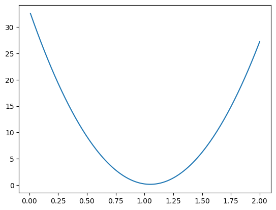
We can now read a reasonable weight from the graph, but update_v0 cannot recognize that it has reached a good solution. It does not even ensure that loss keeps decreasing. We need a better method to guide the parameters toward a minimum, ideally zero when the model can fit the data exactly. That is the subject of the next article.
Summary
This article has focused on one central idea: optimization, the process of adjusting model parameters to minimize or maximize an objective function. It is the mathematical mechanism behind model training.
We started with a simple straight-line model. Later posts will introduce more complex linear models, nonlinear functions, and neural networks. The squared-error objective is the main building block to understand here; we will encounter other objectives later.
What we still lack is an effective update rule. Next, we will implement one of the central optimization algorithms in deep learning: gradient descent.
Next: Part 2: Gradient Descent.