The Little Learner in Python, Part 2: Gradient Descent
Introduction
Welcome to the second article in this series on deep learning from the ground up.
We will pick up the unfinished task from Part 1: The Core Optimization Mechanism. There, we defined a basic linear model, an objective function, and a helper for repeatedly updating parameters. We have not yet implemented an effective optimization algorithm.
Starting with the shape of the objective curve, we will develop gradient descent, one of the central optimization algorithms in machine learning. With an effective update rule, the computer can carry out the learning process itself. We will also try other models to see how general our implementation is—and discover a new problem along the way.
This article reuses line, l2_loss, revise, and the dataset definitions from Part 1. Understanding those functions is essential, so read that article first if you have not already done so. Run its code before working through the examples here.
What a gradient means and how to calculate it
At the end of Part 1, we plotted the objective against the weight $w$:
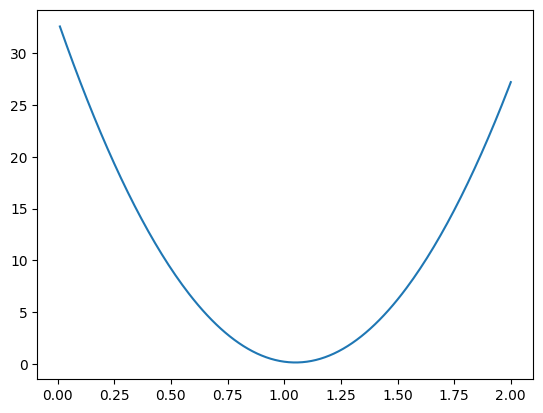
The relationship is a curve, not a straight line. The rate at which the objective changes therefore varies with the parameter value. This helps explain why repeatedly adding a fixed amount such as 0.01 is such a poor update rule: it responds neither to the curve’s slope nor to its direction.
Instead, we can use the objective’s local rate of change to guide both the direction and size of an update. On this bowl-shaped curve, a steeper slope calls for a larger adjustment, while a gentler slope near the bottom calls for a smaller one. For more general objectives, slope alone does not tell us the distance to the best solution, but it still provides useful local information.
Consider a numerical example. At $\theta = [0.0, 0.0]$, the loss is 33.21. Increasing $w$ to 0.0099 while leaving $b$ unchanged gives a loss of 32.5892403, or about 32.59.
Using the unrounded values, the change is:
\[\Delta J = 32.5892403 - 33.21 = -0.6207597\]The estimated rate of change is:
\[\frac{\Delta J}{\Delta w} = \frac{-0.6207597}{0.0099} = -62.703\]This finite difference approximates the instantaneous rate of change: the slope of the tangent to the curve at the starting point. It is not the exact derivative, because we used a nonzero step. With a smaller, suitably chosen step, the approximation approaches the derivative, which is $-63$ here.
Calculate the corresponding rate for every parameter, such as $w$ and $b$, and collect them into a vector. That vector is the gradient. It describes how the objective changes locally as each parameter changes while the others are held fixed.
If you know calculus, these components are the objective’s partial derivatives. The gradient operator is written $\nabla$, pronounced “nabla” or “del.”
Let us calculate one component in Python:
# Use nabla in the name because del is a Python keyword.

def nabla_single(objective_func: Callable[[List[float]], float],
          theta: List[float],
          delta: float = 1e-6) -> float:

    current_loss = objective_func(theta)
    theta[0] = theta[0] + delta
    perturbed_loss = objective_func(theta)
    gradient = (perturbed_loss - current_loss) / delta
    return gradient
delta is the small increment. We approximate the derivative by perturbing the parameter, using the familiar slope calculation $(y_2-y_1)/(x_2-x_1)$. A step that is too large gives a poor local approximation; one that is too small can suffer from floating-point error. We use 1e-6 here. This approach is called numerical differentiation.
This first helper only perturbs the first parameter, and it modifies the supplied list in place. We want a more general version that calculates a component for every parameter. In the next version, each perturbation uses a fresh copy of the original list:
def nabla(objective_func: Callable[[List[float]], float],
          theta: List[float],
          delta: float = 1e-6) -> List[float]:

    current_loss = objective_func(theta)

    def get_grad(theta_copy: List[float], i: int) -> float:

        theta_copy[i] += delta
        new_loss = objective_func(theta_copy)
        return (new_loss - current_loss) / delta

    gradients = [get_grad(theta.copy(), i) for i in range(len(theta))]
    return gradients
It looks more involved, but the structure is straightforward: put the derivative calculation in a helper, then use a list comprehension to apply it to each parameter.
Before moving on, notice the cost. Each partial derivative requires another complete evaluation of the objective. For $n$ parameters, we need $n+1$ forward evaluations: one baseline and one per perturbation. With two parameters this is inexpensive, but with millions it becomes impractical. This limitation is a major reason we will introduce automatic differentiation later in the series.
Now that we can calculate a gradient, we can use it to update the parameters.
The learning rate: controlling the step size
The gradient provides two kinds of local information:
- Direction: moving in the negative-gradient direction decreases a differentiable objective for a sufficiently small step, provided the gradient is nonzero.
- Magnitude: larger components indicate greater local sensitivity to the corresponding parameters.
We still need to decide how far to move. What happens if we simply subtract the gradient?
# Initial parameters.
theta = [0.0, 0.0]

# Calculate the gradient.
grad = nabla(line_objective, theta)  # Approximately [-63.0, -21.0].

# Update directly using the gradient.
theta_new = [theta[0] - grad[0], theta[1] - grad[1]]  # Approximately [63.0, 21.0].

# Calculate the resulting loss.
print(line_objective(theta_new))
The loss jumps to roughly 142,917. It is like trying to leap from a hillside to the valley floor, only to fly across the entire valley and up the opposite side.
To control the step, we multiply the gradient by a small constant. Values such as 0.001 to 0.1 are common starting points, though the appropriate value depends on the problem. This constant is the learning rate, written as the Greek letter $\alpha$.
We will use 0.01 in the following example. Here, scaling the gradient by that amount keeps the updates small enough for the loss to decrease steadily. A learning rate does not guarantee this behavior for every objective; its value matters.
The learning rate is not a model parameter. It controls the optimization process and is chosen separately from the parameters learned from the data. Such settings are called hyperparameters. We have already encountered another one: the number of iterations passed to revise.
How should we choose hyperparameters? For now, we will experiment. More systematic approaches exist, but they are beyond this article. Later, we will touch on a method called grid search.
The update rule can be written as:
\[\theta_{\text{new}} = \theta_{\text{old}} - \alpha \cdot \nabla J(\theta_{\text{old}})\]Here, $\alpha$ is the learning rate and $\nabla J(\theta)$ is the gradient of the objective at $\theta$. Each symbol corresponds to something we have already introduced.
In code:
learning_rate = 0.01

def update_v1(theta: List[float]) -> List[float]:

    # Calculate the gradient.
    gradient = nabla(line_objective, theta)
    # Update each parameter p using its gradient g and the learning rate.
    # This assumes p and g are numbers supporting multiplication and subtraction.
    return [p - learning_rate * g for p, g in zip(theta, gradient)]
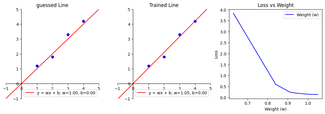
Try the update rule:
theta = revise(update_v1, 1000, initial_theta)
With the code and data shown here, the result is approximately [1.04999736, 0.00000637]: a weight near 1.05 and a bias near zero. This closely matches our visual estimate. The loss falls from 33.21 to approximately 0.135. It does not reach zero because these data points do not all lie on a single straight line.
Implementing gradient descent
We can now combine the helpers into one gradient-descent interface. It should accept an objective, initial parameters, a learning rate, and an iteration count, so that it can work with models other than line.
def gradient_descent(objective_func: Callable[[List[float]], float],
                     initial_theta: List[float],
                     learning_rate: float,
                     num_revisions: int) -> List[float]:

    # The same update rule as update_v1.
    def update(theta: List[float]) -> List[float]:

        grad = nabla(objective_func, theta)

        revised_theta = [p - learning_rate * g for p, g in zip(theta, grad)]
        return revised_theta

    return revise(update, num_revisions, initial_theta)
The inner function is essentially update_v1, but it is now a closure inside gradient_descent. It uses the objective and learning rate passed to the enclosing function instead of global values. Finally, revise applies the update repeatedly.
To test whether the interface works with another model, let us fit a quadratic:
\[y = ax^2 + bx + c\]Here is the Python code:
# Define the model.
def quadratic(xs: Iterable[float]) -> Callable[[float, float, float], List[float]]:

    return lambda a, b, c: [a * x**2 + b * x + c for x in xs]

quad_xs = [-1.0, 0.0, 1.0, 2.0, 3.0]
quad_ys = [2.55, 2.1, 4.35, 10.2, 18.25]

# Start with all parameters at zero.
initial_quad_theta = [0.0, 0.0, 0.0]

# Define the objective.
quad_objective = l2_loss(quadratic)(quad_xs, quad_ys)

# Run gradient descent.
optimized_quad_theta = gradient_descent(
    objective_func=quad_objective,
    initial_theta=initial_quad_theta,
    learning_rate=0.001,
    num_revisions=1000
)

print(f"Quadratic parameters: a={optimized_quad_theta[0]:.4f}, b={optimized_quad_theta[1]:.4f}, c={optimized_quad_theta[2]:.4f}")
Example output:
Quadratic parameters: a=1.4787, b=0.9929, c=2.0546
Plotting the data and fitted curve gives:
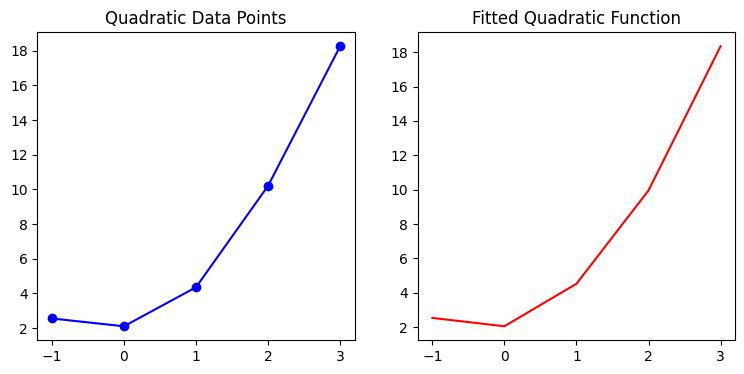
The implementation can fit a curve that is nonlinear in its input. Next, try a linear model with several input features—a plane in the two-feature case:
\[y = w_1x_1 + w_2x_2 + \cdots + w_nx_n + b\]The weight is now a vector:
# A dot product multiplies corresponding values and adds the products.
def dot_product(v1: Iterable[float], v2: Iterable[float]) -> float:

    return sum(x * y for x, y in zip(v1, v2))


def plane(xs: Iterable[Iterable[float]]) -> Callable[[Iterable[float], float], List[float]]:

    return lambda w_vector, b: [dot_product(x, w_vector) + b for x in xs]

# A new dataset.
plane_xs = [(1.0, 2.0), (2.0, 3.0), (3.0, 4.0), (4.0, 5.0)]
plane_ys = [1.0 * x[0] + 0.5 * x[1] + 0.1 for x in plane_xs]

# Initial parameters: a weight vector and a bias.
initial_plane_theta = [[0.0, 0.0], 0.0]


# Define the objective.
plane_objective = l2_loss(plane)(plane_xs, plane_ys)

# Run gradient descent.
optimized_plane_theta = gradient_descent(
    objective_func=plane_objective,
    initial_theta=initial_plane_theta,
    learning_rate=0.001,
    num_revisions=2000
)
# TypeError: 'float' object is not iterable
This raises a type error. Our nabla and update functions assume a flat list of parameters: every element is a number. The plane model instead uses a nested structure, with a list of weights as its first parameter. The implementation does not know how to perturb and update that structure.
You can try modifying nabla and the update function to make this example work. A cleaner, more general solution needs another concept, which we will introduce in the next article.
Interestingly, the corresponding example in the book works at this point. The book introduces operations on nested lists earlier and supplies the differentiation operation through a library rather than implementing numerical differentiation here. This keeps the focus on neural-network concepts. If you know calculus, consider how the chain rule could help calculate derivatives automatically. If you do not, there is no need to worry: a later article will explain automatic differentiation and implement it.
Summary
Gradient descent combines three steps:
- Calculate the gradient to determine a local direction of improvement.
- Scale it by the learning rate to control the update size.
- Repeat the update to move toward a minimum.
We successfully used the same interface to fit both a straight line and a quadratic curve. You have now seen the full process of training a simple model by learning its parameters.
This is only a basic gradient-descent implementation. Later posts will explore variants and improvements, as well as how all of this connects to neural networks and deep learning.
The immediate problem is that our list-based helpers cannot handle nested parameter arrays. We could patch the functions for this one example, but a general solution would be more useful. The next article introduces tensors and develops operations that work with higher-dimensional data.
For now, take a break.
Previous: Part 1: The Core Optimization Mechanism.
Next: Part 3: Tensors (Chinese).